The economic forces underpinning the above findings are perhaps best explained through basic supply and demand analysis. Consider the below chart on this issue.
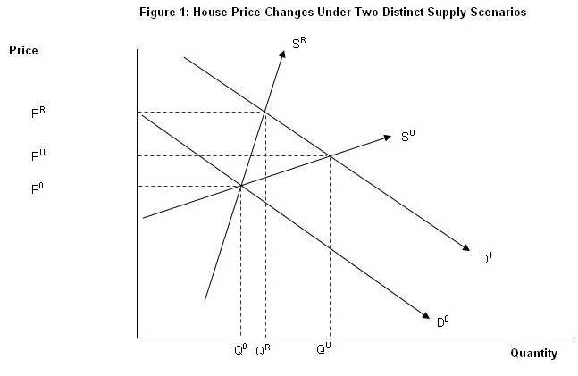
Q0 and P0 represent the initial equilibrium situation in the housing market. Initial demand is provided by D0, whereas supply is shown as either SR (restricted) or SU (unrestricted), depending on whether land supply constraints exist.
Following an increase in demand, such as that brought about by a significant relaxation of lending standards, the demand curve shifts outwards from D0 to D1. When land supply is restricted, house prices rise sharply from P0 to PR. By contrast, when supply is unrestricted, prices rise more gradually from P0 to PU.
The situation works the same way in reverse. For example, if there was a sharp fall in demand following a contraction in credit availability or a sharp rise in unemployment, causing demand to fall from D1 to D0, then prices fall much further when land supply is constrained.
The key point is that increases (declines) in demand can bring sharply rising (falling) house prices when supply is constrained. However, when land supply is not regulated, it adjusts to demand and house price volatility is reduced.